
In late March, the Supreme Court will hear a case where Republican voters argue that Maryland’s Sixth Congressional District is an unconstitutional partisan gerrymander.
Maryland defends the map, saying that legitimate considerations related to the historical configuration of the district drove decisions about district boundaries. But there are good reasons to be suspicious of that claim, on its face. The biggest of these is simply the extremeness of the changes made to the existing district.
The Sixth District was overpopulated by about 17,414 people as Maryland started the 2010 redistricting cycle.[1] But we estimate that Democratic map drawers, rather than tweak the district at the edges to achieve the population parity that the Constitution requires, moved a total of 711,162 people into or out of the district (that’s 353,088 people moved into the district and 358,074 people moved out).[2] That’s more than 40 times the number needed to meet population equality requirements.
To gauge how that population shift compares with changes made in other districts around the country, the Brennan Center analyzed needed versus actual population shifts for every congressional district in the United States. The results were extraordinary.
An earlier study, by Antoine Yoshinaka and Chad Murphy, found that members of the out-of-power party tended to have more drastic changes made to their districts as a way for the in-power party to insulate its members.[3] But our analyses show that what happened in Maryland’s Sixth District was well outside the norm. Only 7 of 132 districts in comparable states saw changes as extreme as that in the Maryland Sixth. And five of those were in North Carolina, where an aggressive racial gerrymander of the state’s congressional map was struck down by the Supreme Court in 2016.
By almost any measure, the Maryland Sixth is an outlier. We show where the Maryland Sixth falls relative to all the districts that were redrawn after the 2010 census, and then in relation to slices Yoshinaka and Murphy identified as significant in their study: among districts that are a similar distance from population equality or among similarly populated states.
Needed versus Actual Changes to Districts: The National View
One of the main legal requirements of redistricting is to redraw electoral districts so that districts have the same number of constituents.[4] For most districts, this is a small undertaking. We estimate that, excluding the seven at-large districts, an average of 59,976 people needed to be moved in or out of a district in 2011 to achieve population equality. The Maryland Sixth District, needing just 17,414 people, was well below this average.
As Figure 1 shows, in states that did not gain or lose a congressional district (with the exception of California and, to a lesser extent, North Carolina), the changes made to achieve population equality tended to be roughly proportional to the number of people that needed to be moved. In other words, if a district needed to lose 10,000 people then somewhere around 10,000 people were moved out of the district. In short, states were minimalists, changing districts as little as possible.
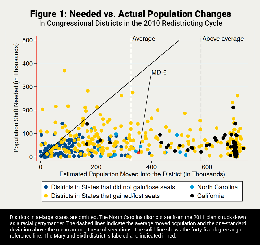
The main exception among states where the number of districts stayed the same was California, where a newly created independent commission undid an infamous bipartisan gerrymander that had used “mangled lines” to make every seat a safe seat regardless of party.[5] The new map “radically, and more logically, rearranged the state’s 53 seats” and resulted in a higher-than-average number of moves. The other noteworthy exception was North Carolina, where Republicans, after gaining control of the redistricting process for the first time since Reconstruction, “painstakingly packed Democratic voters into just three of the state’s 13 seats.”[6] Here, too, large numbers of people were moved in and out of districts despite the fact the size of North Carolina’s congressional delegation remained the same.
Not surprisingly, changes also were more extensive if a state gained or lost congressional districts. When this happened, even districts that needed to add or lose only a small number of people sometimes shifted considerably to accommodate the increased or decreased number of districts. The yellow dots in Figure 1 indicate that a change in the size of a state’s congressional delegation has a pronounced effect on the population shifts within the state. The previous study by Yoshinaka and Murphy found this to be the case in the 2000 redistricting cycle as well.
Even viewed at the national level, Maryland’s Sixth District stands out. Although it is in the middle of the pack among all districts, almost all districts where a greater number of people were moved were either in states that gained or lost a congressional seat or in California, where a gerrymander was being unwound.
Drilling Down: Changes to Districts in Comparable States
When we omit districts in the states that gained or lost a district and in California (Figure 2), and focus on states where the number of districts stayed the same, the aggressiveness of the changes to the Maryland Sixth becomes even clearer.
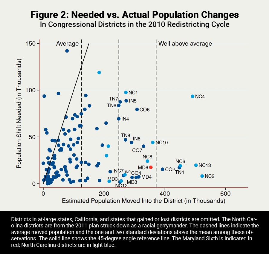
In this set of 132 comparable districts, the Maryland Sixth is almost two standard deviations above the mean in terms of the population that was moved into the district during the 2010 redistricting cycle. In this set of cases, there are only seven districts that moved more people—on an absolute basis—than the Maryland Sixth. Put another way, the Maryland Sixth moved more people into the district than 94 percent of the comparable districts in the country. Of the districts that moved more people, five of them are in North Carolina’s racially gerrymandered map.
Indeed, the only districts not in North Carolina where more people were moved were the Colorado Second District, which was drawn by a court after legislative deadlock, and the Tennessee Fourth District, which was drawn by a Republican legislative trifecta.
Drilling Down Further: Changes to Districts Needing Similar Levels of Population Adjustment
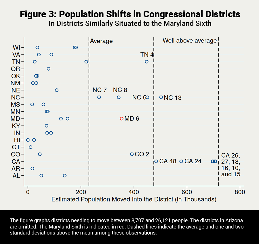
We confirm our observations about the Maryland Sixth by looking at districts in comparable states that had to move between 50 percent and 150 percent of the number that needed to be added to the Maryland Sixth. As Figure 3 shows, out of 44 districts in this category, only three districts, once we set aside the California and North Carolina cases, had a higher number of moves than the Maryland Sixth. Even counting California districts, the Maryland Sixth still ranks in the top third. We depart from Yoshinaka and Murphy’s research design by including districts from California here.[7] Our intention is to demonstrate the extent to which the independent redistricting commission worked to remove the bipartisan gerrymander in that state.
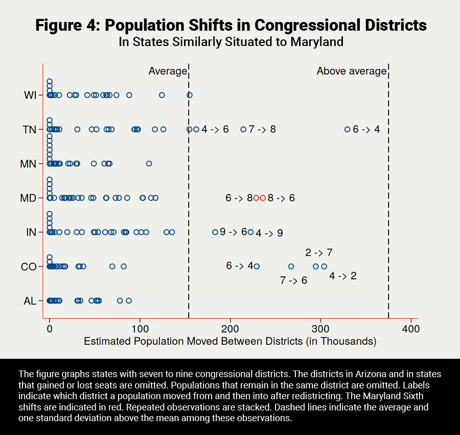
Yoshinaka and Murphy noted that states with a larger U.S. House delegation tend to see more disruption to districts, and we wanted to reduce the possibility that this factor would skew our analyses of the Maryland Sixth District. Therefore, Figure 4 shows population movement only for states with seven to nine congressional seats, comparable to Maryland’s eight. It is apparent from this figure that the changes to the Maryland Sixth were not only unusual among states but unusual within Maryland. Most of Maryland saw minimal population movement between districts in the 2011 round of redistricting. By contrast, the shifts between the Sixth and Eighth Districts stand out. They are far larger than any other shifts in Maryland, and also exceptional among similar-size states. In total we report 276 observations in this slice of data. The two indicated observations from Maryland are the 16th and 18th in order of the population shift, or more extreme than 94 percent of the other observations in the figure.
In sum, the Maryland Sixth is an example of a district that deserves close examination to ensure that district lines were not redrawn purely on the basis of partisan motives.
Appendix: Methodology
We used a variety of data from the 2010 U.S. Census in the analyses we conducted for this report. We began with the total population estimates for each block group in the United States. Census data are aggregated at different geographic levels, from small units like neighborhoods to the country as a whole. The most granular unit of geography in the U.S. Census is the census block, a unit of area defined as bounded by visible features (e.g., a street) and nonvisible boundaries, like property lines and city limits.[8] There are more than 11 million census blocks in the 50 states and the District of Columbia. Census blocks are nested within block groups, the second-most granular layer of aggregated Census data and the basis of our analyses here. A block group is a contiguous statistical division of a census tract and generally contains between 600 and 3,000 people.[9] There are 217,740 block groups in the United States, excluding Puerto Rico and the Island Areas.[10]
Once we had counts of the total population in each block group, we joined this data with a map of block groups in each state. The U.S. Census has produced geographical information systems (GIS) data since the 1990 Census as part of its TIGER database.[11] These GIS files allow researchers to assign a given data point to a location in space to then relate it to other points in space. For example, the total population of the first block group within the first census tract of Allegany County in western Maryland is 826. We can add this unit of geography together with other block groups to divide Maryland into congressional districts.[12] The Census Bureau’s TIGER database includes the necessary data files to define each congressional district in the United States and then to project those shapes on a computer-based map. For our purposes, the congressional districts in the 111th Congress (which sat from January 2009 to January 2011, following the 2008 elections) and 113th Congress (in session from January 2013 to January 2015, following the 2012 elections) allowed us to estimate the pre- and post-redistricting population in each congressional district.
We accounted for the populations moved around in the course of the redistricting process using the districts as a sort of bookend. We overlaid a map of the congressional districts as they were configured in the 2010 elections on top of the map of block groups in each state to assign a block group to one district (or more than one, if a block group is split).[13] We then repeated the same process using the map of districts as they were configured in the 2012 elections to assign each block group to a district (or districts). By comparing the 2010 district number with the 2012 district number, we could separate the populations that stayed in the same district from those that moved from one district to another. These population estimates were then directly incorporated into our analyses of different slices of the data from each congressional district in the graphics we show and discuss.
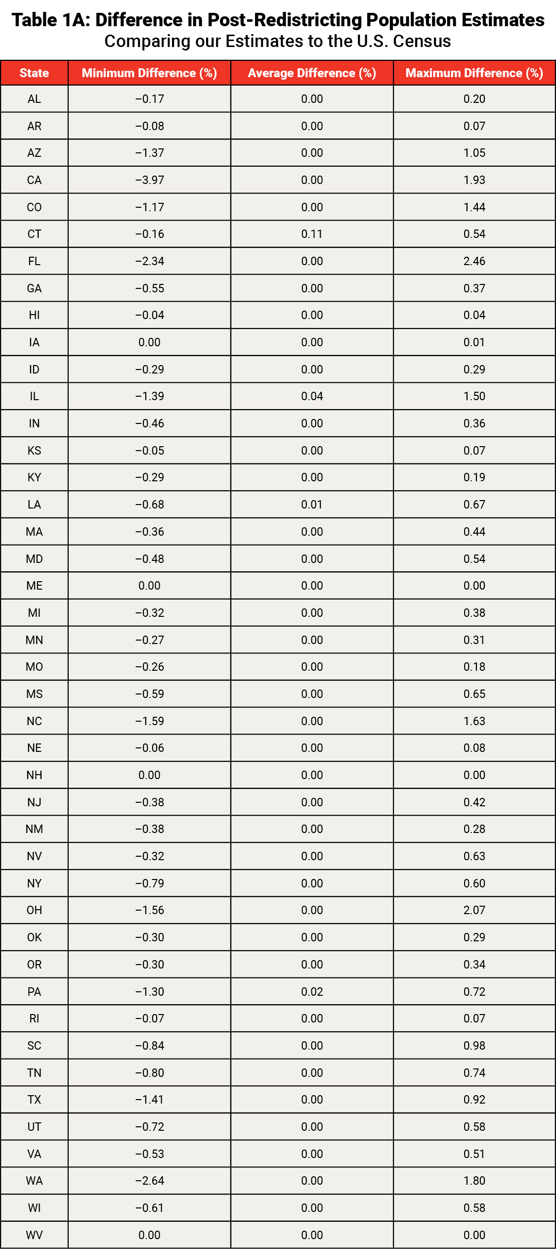
This procedure allowed us to assess the accuracy of our population estimates. The U.S. Census provides official pre- and post-redistricting counts of the total population of each congressional district.[14] In the table below, we compare our post-redistricting population estimate for states with more than one congressional district to the numbers provided by the U.S. Census. We report the minimum, average, and maximum percentage difference between our district population estimate and the official post-redistricting population enumeration. Our estimates are, on average, within about one-tenth of one percentage point of the official count in each state. At the district level, our estimates are no more than about 4 percentage points below the officially reported quantity and no more than 2.5 percentage points above the official report. Our estimates are somewhat less accurate as the number of congressional districts increases, but they do not rise to the point of markedly deviating from the official reports. The analyses we present in this report follow from these data, a combination of official Census figures and our supplements to these population counts.
[1] This difference in population was calculated on the basis of pre- and post-redistricting total populations reported for the district. The U.S. Census reported that the pre-redistricting total population in the Sixth District was 738,943. The General Assembly of Maryland reported that the post-redistricting population, after adjusting the numeration to account for institutionalized persons, of the Sixth District was 721,529. General Assembly of Maryland, County Population Totals by District, October 2011, http://mlis.state.md.us/Other/Redistricting/gracsb1hb1countypop.pdf.
[2] We describe the methodology leading to this estimate in an appendix that follows our analyses. We estimate much of the population that moved out of the Sixth District after 2010 ended up in the Eighth District, and smaller portions moved to the First, Seventh, and Second Districts. Populations that moved into the Sixth District after 2010 originated in the Eighth and Fourth Districts.
[3] Antoine Yoshinaka and Chad Murphy, “Partisan Gerrymandering and Population Instability: Completing the Redistricting Puzzle,” Political Geography 28 (2009): 451–462, https://doi.org/10.1016/j.polgeo.2009.10.011.
[4] The initial claim in the 1962 Supreme Court case Baker v. Carr, from which much of the redistricting jurisprudence is descended, was that the Tennessee legislature had not reapportioned itself in the 61 previous years, to the point that Justice Brennan, writing for the majority, observed that “the State Senator from Tennessee’s most populous senatorial district represents five and two-tenths times the number of voters represented by the Senator from the least populous district, while the corresponding ratio for most and least populous House districts is more than eighteen to one.” The Court departed from previous practice and signaled that the judiciary could step in to curb excesses in redistricting.
[5] Michael Barone and Chuck McCutcheon, The Almanac of American Politics 2014 (Chicago: University of Chicago Press, 2013), 129. The legislature-drawn plan in California is an example of a bipartisan gerrymander designed to insulate incumbents. In 2002, for example, “[t]he smallest margin of victory for any California congressional incumbent was 18 percentage points, and the average incumbent received a 68 percent vote share.” See Richard Forgette and Glenn Platt, “Redistricting Principles and Incumbency Protection in the U.S. Congress,” Political Geography 24 (2005): 934–951, https://doi.org/10.1016/j.polgeo.2005.05.002. The map in California was also durable. In the elections between 2002 and 2010, only one U.S. House seat changed parties.
[6] Barone and McCutcheon, The Almanac of American Politics 2014, 1233.
[7] Yoshinaka and Murphy observe, “If large inter-district population shifts produced by redistricting can alter an incumbent’s career and reelection prospects, it is only natural to expect partisan mapmakers to use this tool strategically, and foster more instability for some incumbents than for others” (see Yoshinaka and Murphy, “Partisan Gerrymandering and Population Instability,” 452). The use of this tool by nonpartisan institutions like courts or independent commissions is less well known in the academic literature.
[8] See https://www.census.gov/geo/reference/gtc/gtc_block.html for the definition of a census block.
[9] See https://www.census.gov/geo/reference/gtc/gtc_bg.html for the definition of a block group.
[10] See https://www.census.gov/geo/maps-data/data/tallies/tractblock.html for a tally of census tracts, block groups, and blocks for each state and territory within the United States.
[11] The TIGER database is available at https://www.census.gov/geo/maps-data/data/tiger.html.
[12] ESRI, Inc., the major developer and distributor of GIS data and software, has created a training module to familiarize users with its GIS software by drawing congressional districts in Maryland using Census and geographic data: https://learn.arcgis.com/en/projects/redraw-political-boundaries-with-public-participation.
[13] We made an assumption that the population of block groups is uniformly distributed within the block group. In cases where a block group is split, we estimated the population of each segment of the block group by multiplying the total population of the block group by the ratio of the area of the segment of the block group to the area of the whole block group. For example, if a block group covers 100 square miles, has 100 people in it, and is equally split between two districts, we assigned a population of 50 to each district.
[14] Pre-redistricting total population estimates by congressional district are available at https://factfinder.census.gov/bkmk/table/1.0/en/DEC/10_SF1/P1/0100000US.50000.111. Post-redistricting total population estimates by congressional district are available at https://factfinder.census.gov/bkmk/table/1.0/en/DEC/10_113/P1/0100000US.50000.113.